11.4. General Persistence Diagrams

Persistence diagrams (and barcodes) give a visual representation of how a filtration of a topological space (usually a simplicial complex) evolves. It keeps track of homological dimensions which are "born" and "killed" throughout this evolution.

Let \(X\) be a topological space. We know from algebraic topology that there exists a \(n\)-th singular homology group

\[ H_n(X). \]

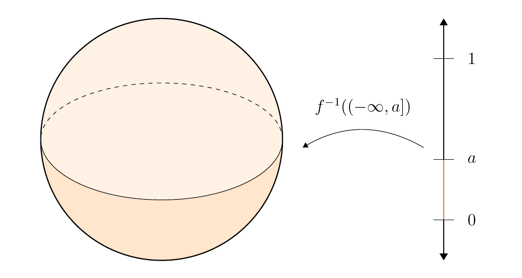
Suppose that \(f: X \to \mathbb{R}\) is a real-valued function. An example of this is the height function of a sphere centered at the origin. Now one thing we can do with these types of functions is take any \(a \in \mathbb{R}\) and consider

\[ f^{-1}((\infty,a]) \subset X. \]

The space \(f^{-1}((\infty,a]) \subset X\) is a topological space induced by the subspace topology of \(X\). In general, this process can be modeled functorially. Let \(\mathbb{R}\) be a category with morphisms given by poset structure. Then

\[\begin{align*} &E: \mathbb{R} \to **Top**\\ &a \longmapsto f^{-1}((\infty, a]) \end{align*}\]

since if \(a \le b\) then this induces a continuous function

\[ i: f^{-1}((\infty, a]) \to f^{-1}((\infty, b]) \]

namely, the inclusion function. \textcolor{NavyBlue}{We denote the functor as \(E\) for "evolution," as this functor filters the space \(X\). As we send \(a\) to infinity, we ultimately obtain the entire topological space.}

Switching focus, consider the homology group of this subspace

\[ H_n(f^{-1}((\infty, a])). \]

We can also outline this behavior as functorial where we send

\[\begin{align*} &H: **Top** \to **Ab** \\ &f^{-1}((\infty, a]) \longmapsto H(f^{-1}((\infty, a])) \end{align*}\]

since for any \(a \le b\), we have a group homomorphism which we denote as \(\phi_a^b\):

\[ \phi_a^b: H(f^{-1}(\infty, a]) \to H(f^{-1}(\infty, b]). \]

Now we can outline this overall data pipeline as a functor \(H \circ E: \mathbb{R} \to **Ab**\)

\[\begin{align*} &H \circ E: \mathbb{R} \to **Top** \to **Ab** \\ & a \longmapsto f^{-1}((\infty, a]) \longmapsto H(f^{-1}((\infty, a])). \end{align*}\]

What's really happening here? First, \(E\) records the evolution of the topological space under \(f: X \to \mathbb{R}\). Then \(H\) records the homology groups; overall, \(H \circ E\) records the topological evolution! We are thus interested in the following objects.

Let \(a \le b\). Recall that

\[ H\circ E(a \le b) = \phi_a^b. \]

Since we are interested in the image of these mappings, which will be a group, we denote

\[ F([a, b]) = \im(\phi_a^b) = \im\Big( H(f^{-1}((\infty, a ])) \to H(f^{-1}((\infty, b])) \Big) \]

to be a persistence homology group from \(a\) to \(b\).

For a persistence homology group \(F([a, b])\), define the Betti number from \(a\) to \(b\) as

\[ \beta_a^{b} = \text{rank}(F([a, b])). \]

In most nice topological spaces, the homology doesn't change much through its evolution. That is, as we move from \(a\) to \(b\), the persistence homology groups \(F_a^b\) don't change much.

For example, if \(f: X \to \mathbb{R}\) is the height function and \(X\) is a sphere, the topology will not change until we get from one pole to the other.

\textcolor{NavyBlue}{What does it mean for the topology to change in this context}? It means that we were at some value \(a\), but then at \(a +\epsilon\) the homology became different. This means that

\[ H(f^{-1}((\infty, a])) \to H(f^{-1})(\infty, a + \epsilon] \]

is not an isomorphism. Finding out when the homology does change is valuable information, so we keep track of these points.

A critical value of \(f: X \to \mathbb{R}\) is an \(a \in \mathbb{R}\) such that there exists an \(\epsilon > 0\) such that

\[ H_n(f^{-1}((\infty, a - \epsilon])) \to H_n(f^{-1}((\infty, a +\epsilon ])) \]

is not an isomorphism. The function \(f\) is called tame if \(f\) has finitely many critical values. \

Let \(f: X \to \mathbb{R}\) be a tame function. Then we have finitely many critical values \(\{s_1, s_2, \dots, s_n\}\). Let \(\{t_0, t_1, \dots, t_{n}\}\) be any interleaved sequence of numbers such that \(t_{i-1} < s_i < t_{i}\). We will see soon why such a choice has much freedom in it. Now append to this sequence \(t_{-1} = s_0 = -\infty\) an \(t_{n+1} = s_{n+1} = \infty\).

We are now ready to define persistence diagrams. \ \

Let \(f: X \to \mathbb{R}\) be tame and \((s_i, s_j)\) be a tuple of critical values. Then we define the multiplicity of \((s_i, s_j)\) to be

\[ \mu_{i}^{j} = \beta_{t_{i-1}}^{t_i} -\beta_{b_i}^{b_j} + \beta_{b_{i}}^{b_{j-1}} - \beta_{b_i}^{b_j} \]

The persistence diagram of the tame function \(f: X \to \mathbb{R}\) \(D(f)\) is the multiset of tuples \((s_i, s_j)\) each with multiplicity \(\mu_i^j\). Alternatively,

\[ D(f) = \bigcup_{i=0}^{n+1}\bigcup_{j = 0}^{n+1} \left( \bigcup_{k = 1}^{\mu_i^{j}} \{ (s_i, s_j) \}\right) \]

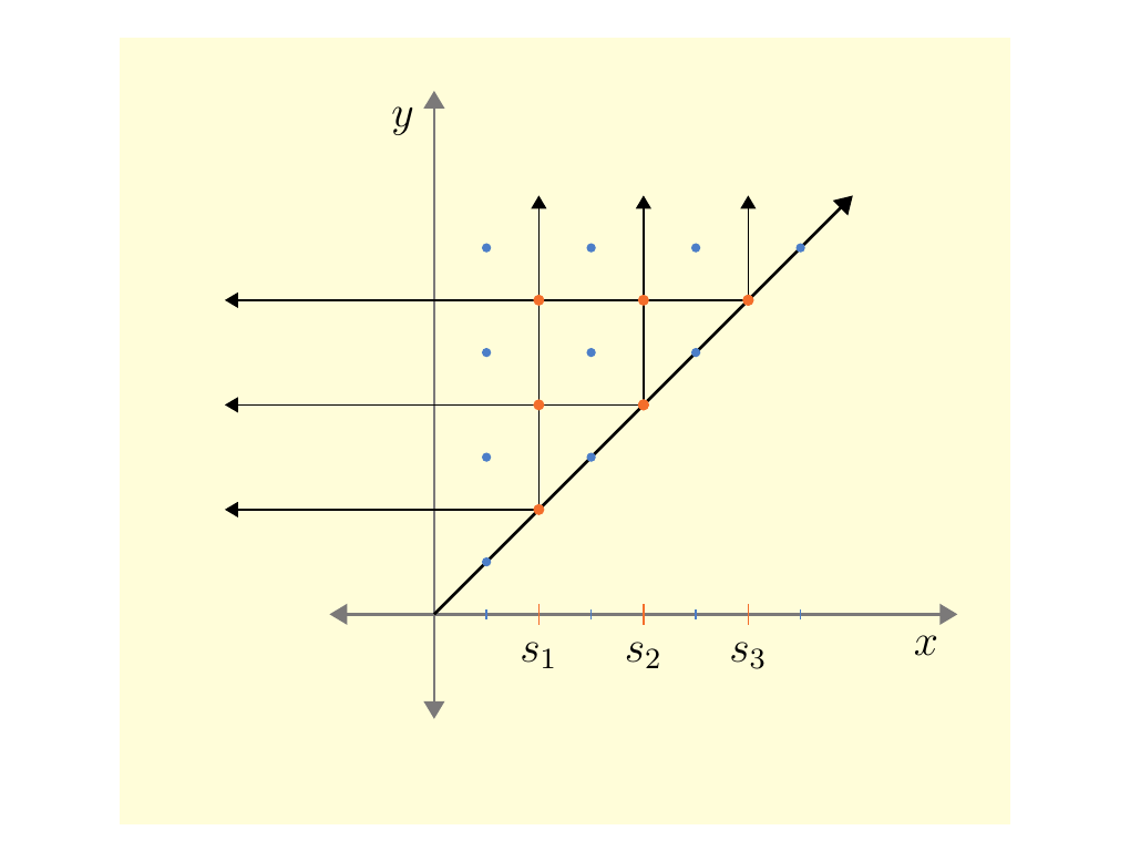
Persistence diagrams consist of points in \(\rr \times \rr \cup\{\infty\}\) above the diagonal \(y = x\). Thus let \(**Dgm**\) be the category of half open intervals \([p, q)\) with \(p < q\) and intervals of the form \([p, \infty)\).

In what follows, let \(S = \{s_1, s_2, \dots, s_n\}\) be a finite set of real numbers, and let \((G, +)\) be an abelian group with identity \(e\).

A map \(X: **Dgm** \to G\) is \(S\)-constructible if for every \(I \subset J\) where

\[ J \cap S = I \cap S \]

we have \(X(I) = X(J)\). The motivation for defining this type of function arises from the rank function

\[\begin{align*} \beta_a^b&:**Dgm** \to \mathbb{Z}\\ &= \text{rank}(F([a, b]))\\ &= \text{rank}(\im\Big( H(f^{-1}((\infty, a ])) \to H(f^{-1}((\infty, b])) \Big)) \end{align*}\]

Suppose that our critical points are \(S = \{s_0, s_1, s_2, s_3\}\) and that we have two intervals \(I = [a, b]\) and \(J = [c, d]\) such that \(I \subset J\) and \(I \cap S = J \cap S\).

Clearly in this case we have that \(I \cap S = J \cap S\). Now observe that

\[ \beta_a^b = \beta_c^d \]

since these intervals observe the same changes in rank.

\textcolor{NavyBlue}{Therefore, we see that the rank function for a tame function \(f: \mathbb{R} \to X\) is \(S\)-constructible.}

A map \(Y: **Dgm** \to G\) is \(S\)-finite if

\[ Y(I) \ne e \implies I = [s_i, s_j) \text{ or } I = [s_i, \infty) \]

Alternatively, this states that

\[ I \ne [s_i, s_j) \text{ and } I \ne [s_i, \infty) \implies Y(I) = e. \]

which is probably a better way of thinking about this.

This leads to the following definition:

A persistence diagram is a finite map \(Y: **Dgm** \to G\).

The motivation for this is due to the persistence diagram. Given a persistence diagram, we can extend it to a mapping

\[\begin{align*} &X: **Dgm** \to \mathbb{Z}\\ &[a, b) \mapsto \beta_{a_1}^{b_1} - \beta_{a_2}^{b_2} + \beta_{a_2}^{b_1} - \beta_{a_1}^{b_1} \end{align*}\]

where \(a_1 \le a \le a_2\) and \(b_1 \le b \le b_2\) are values within some sufficiently small neighborhood of \(a\) and \(b\). Note that in this extension, if \([a, b) \ne [s_i, s_j)\) or \([s_i, \infty )\) in, then each \(\beta_{a_i}^{b_j}\) is of full rank, so that

\[ X([a, b)) = 0. \]

Hence we see that the persistence diagram is \(S\)-finite where \(S\) is the finite set of critical values.

We now want to invent a distance between persistence diagrams. To do so, we must first denote \(G\) as not only an abelian group, but one with a translational invariant partial ordering \(\le\). What we mean by that is if \(a \le b\) then \(a + c \le b + c\) for any \(a, b ,c \in G\).

Consider \(Y_1, Y_2: **Dgm** \to G\) be a pair of persistence diagrams. We say there exists a morphism \(\phi: Y_1 \to Y_2\) if

\[ \sum_{\substack{J \in **Dgm** \\ I \subset J}}Y_1(J) \le \sum_{\substack{J \in **Dgm** \\ I \subset J}}Y_2(J) \]

for all \(I \in **Dgm**\).

Note the above sums are finite.

\textcolor{NavyBlue}{Observe that if \(\phi: Y_1 \to Y_2\) and \(\phi': Y_2 \to Y_3\), then we can define the unique morphism \(\phi' \circ \phi : Y_1 \to Y_3\). Therefore, this morphism relation establishes a reflexive, transitive ordering on our persistence diagrams.} Thus we can consider the category of persistence diagrams \(**PDiag**(G)\) into the group \(G\) where the objects are persistence diagrams \(Y: **Dgm** \to G\) and morphisms as described above. As we stated before, these morphisms make this category into a partial ordering.

Define the mapping

\[\begin{align*} **Grow**_\epsilon: **Dgm** &\to **Dgm**\\ [p, q) &\mapsto [p - \epsilon, q + \epsilon] \text{ and } [p, \infty) \mapsto [p - \epsilon, \infty). \end{align*}\]

Now consider a pair of persistence modules \(Y_1, Y_2: **Dgm** \to G\). Since they are persistence modules, we know by definition that they are \(S_1\) and \(S_2\)-finite for some finite sets \(S_1, S_2\). With that said, observe that \(Y_1 \circ **Grow**_\epsilon, Y_2 \circ **Grow**_\epsilon: **Dgm** \to G\) are again persistence modules since they \(S_1'\) and \(S_2'\) finite, where\dots

Therefore, we have an endofunctor on our category of persistence modules.

\[\begin{align*} \nabla_\epsilon : **PDgm**(G) \to **PDgm**(G)\\ Y_1: **Dgm** \to G \mapsto Y_1 \circ **Grow**_\epsilon: **Dgm** \to G. \end{align*}\]

Note that for any persistence modules \(Y: **Dgm** \to G\), we have that \(\nabla_\epsilon(Y) \to Y\) since for any interval \(Y\),

\[ \sum_{\substack{J \in **Dgm** \\ I \subset J}}Y(J) = Y_1 \circ **Grow**_\epsilon \]