Vanishing Gradients in RNNs and LSTMs

Recurrent neural networks (RNNs), which can be thought of as feedforward neural networks with self-connections, perform extremely well for supervised sequence learning and are capable of solving many problems that feedforward neural networks typically cannot solve. However, in the past, RNN training procedures suffered from the vanishing gradient problem. This problem led to the invention of the Long Short-Term Memory (LSTM) model. In this work, we review the vanishing gradient problem for vanilla RNNs, and show how the LSTM is able to address this problem. To do this, we offer closed-form gradient update formulae which allow us to mathematically analyze network loss.

Recurrent Neural Networks

Recurrent neural networks are a recursively-defined neural network which sequentially processes a sequence of inputs to produce a corresponding sequence of outputs. The architecture of a RNN generally consists of an input layer with \(I\)-many nodes, a hidden layer of \(H\)-many nodes which have self-connections, and a output layer with \(K\)-many nodes. With such a network, we can iteratively process a sequence of inputs \((x_1, x_2, \dots, x_T)\) with \(x_i \in \mathbb{R}^{I}\), and produce a corresponding sequence of values \((y_1, \dots, y_T)\). This process is described as follows.

We follow a notation system introduced by (Graves, 2012). Specifically, let \(x_i^{t}\) denote the \(i\)-th element of the \(t\)-th input and let \(y_k^{t}\) denote the \(k\)-th element of the \(t\)-th output. Let \(a_j\) denote the network input to network node \(j\) and let \(b_j\) be the activation of node \(a_j\). Moving forward, \(w_{ij}\) will denote the weight going from node \(i\) to node \(j\), and \(\theta\) will denote a differentiable activation function.

With this notation system, the equations that characterize the forward pass of a sequence \((x_1, \dots, x_T)\) for a RNN are as below.

\[\begin{align} a_h^{t} &= \sum_{i = 1}^{I}w_{ih}x_i^{t} + \sum_{h'=1}^{H}w_{h'h}b_{h'}^{t-1}\\ b_h^{t} &= \theta(a_h^{t})\\ a_k^{t} &= \sum_{h=1}^{H}w_{hk}b_h^{t}\\ y_k^{t} &= \theta(a_k^{t}) \end{align}\]

Computing the forward pass requires starting at \(t = 1\) and incrementing until \(t = T\). Note that this requires an initial value for \(h_0\), which we initialize to the zero vector.

Example RNN

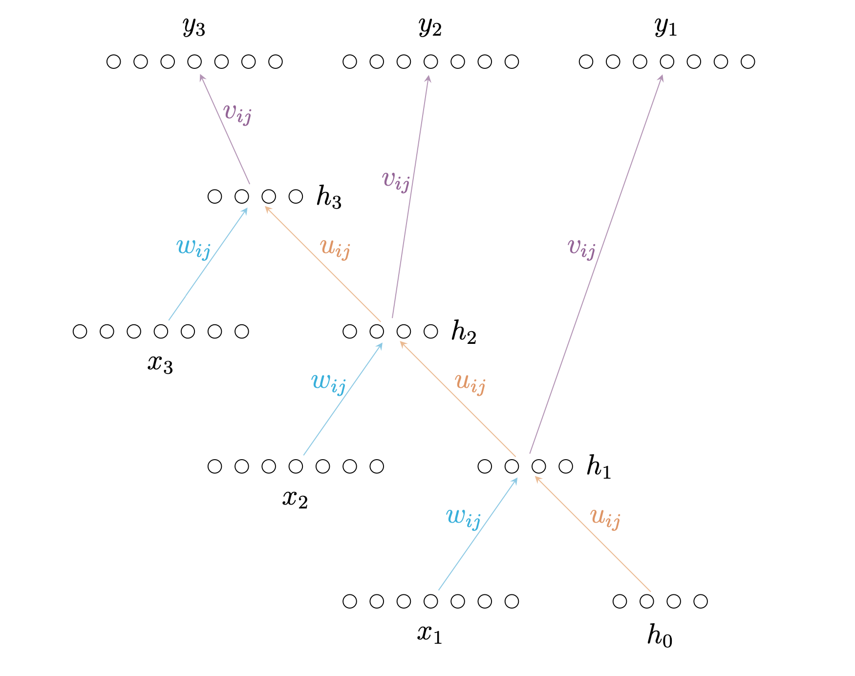
To make things concrete, let us introduce a simple example of a recurrent neural network. For our network architecture, set \(I = K = 7\), so that the input and output of the RNN are in \(\mathbb{R}^7\), and set \(H = 4\), so that the hidden states are in \(\mathbb{R}^4\). This is what the RNN looks like.

As a side note, this RNN is capable of perfectly learning the Reber grammar.

Notation

The notation we introduced is using a notation strategy from Graves' work, and it is technically an abuse of notation with respect to the weights. However, the idea is that it is generally clear from context what layer in the network \(w_{ij}\) will refer to. When we write \(w_{hk}\), we are speaking of the weight connecting node \(h\) in the hidden layer to node \(k\) in the output layer. When we write \(w_{ih}\), we are speaking of the weight connection node \(i\) in the input layer to node \(h\) in the hidden layer. When it is not clear from context we will explicitly state what exact nodes \(w_{ij}\) is connecting.

We now turn to discussion of the backward pass of RNNs. There are several methods one can employ to perform the backward pass, but we will focus on the most common, which is Backpropagation Through Time.

Backpropagation Through Time

The Backpropagation Through Time (BPTT) algorithm is simply an application of the standard backpropagation algorithm for feed-forward neural networks to RNNs. This can be done because RNNs can be viewed as feed-forward RNNs, by "unfolding" the network. This is similar to how a recursive function in programming can viewed as non-recursive function; the logic performed by a recursive function call can equally be performed by one single call to an equivalent non-recursive function.

For example, suppose we processed three elements \((x_1, x_2, x_3)\) through the RNN we introduced earlier. Then the network unfolded would look like this:

Well actually, what it would really look like is something like this:

Thus, we can apply standard backpropagation to the unfolded network.

Let \(\mathcal{L} : \mathbb{R}^{I} \times \mathbb{R}^{K} \to \mathbb{R}\) denote the loss function for our supervised training. The function takes in an input and a corresponding known output value to compute a loss value.

The goal of BPTT is to compute the gradient

\[ \frac{\partial \mathcal{L}}{\partial w_{ij}} \]

for all weights \(w_{ij}\) in our network. When this quantity is known, we can update our weights via

\[ w_{ij} = w_{ij} - \eta\frac{\partial \mathcal{L}}{\partial w_{ij}} \]

where \(\eta\) is our learning parameter. Of course, we can also incorporate momentum.

To compute the gradient, note that for a sequence of inputs \((x_1, \dots, x_T)\) with known outputs \((z_1, \dots, z_{T})\), each \(w_{ij}\) in the network contributes loss at each time step. Therefore,

\[ \frac{\partial \mathcal{L}}{\partial w_{ij}} = \sum_{t = 1}^{T} \frac{\partial \mathcal{L}}{\partial a^{t}_j} \frac{\partial a^{t}_j}{\partial w_{ij}} \]

If we introduce the shorthand

\[ \delta_{j}^{t} = \frac{\partial \mathcal{L}}{\partial a^{t}_j} \]

then we have that \(\frac{\partial \mathcal{L}}{\partial w_{ij}} = \sum_{t = 1}^{T} \delta_j^{t} \frac{\partial a^{t}_j}{\partial w_{ij}}\).

In the above expression, \(w_{ij}\) is a general weight in our network. Since there are three different types of layers in our network, there are three different types of weights in the network. We briefly summarize the values of \(\frac{\partial \mathcal{L}}{\partial w_{ij}}\) in each case. If \(w_{ij}\) is a weight connecting an input node to a hidden node, then

\[ \frac{\partial \mathcal{L}}{\partial w_{ij}} = \sum_{t = 1}^{T} \delta_j^{t} x_i^{t} \]

If \(w_{ij}\) is a weight connecting a hidden node to a hidden node, then

\[ \frac{\partial \mathcal{L}}{\partial w_{ij}} = \sum_{t = 1}^{T} \delta_j^{t} b_i^{t-1} \]

If \(w_{ij}\) is a weight connecting a hidden node to an output node, then

\[ \frac{\partial \mathcal{L}}{\partial w_{ij}} = \sum_{t = 1}^{T} \delta_j^{t} b_i^{t} \]

Therefore, to compute BPTT, all that is left to compute is \(\delta_j^{t}\). With RNNs, the network input to node \(h\) in the hidden layer at time \(t\) affects not only all of the values \(y_k^{t}\), but also all of the values in the hidden layer at time \(t + 1\). Therefore, we have the following recurrence relation

\[ \delta^{t}_j = \theta'(a^{t}_j) \left(\sum_{k =1}^{K}w_{jk}\delta_k^{t} + \sum_{h =1}^{H}w_{jh}\delta_h^{t + 1}\right) \]

If we set \(t = T + 1\), note that \(\delta_h^{T+1} = 0\) because the hidden layer values at timestep \((T+1)\) have no effect on the loss. Using this as an initial value, we can then calculate all values of \(\delta_j^{t}\) starting with \(t=T\) and decrementing \(t\) until reaching \(t = 1\).

Vanishing Gradients in BPTT

The BPTT algorithm we described earlier can be easily programmed into a computer and used to train a RNN. However, what one will notice for long sequences is that the RNN will not be able to remember features if there are long gaps between them in the training data. Or, the RNN will have difficulty converging. This is a problem was identified by many researchers in the 1990s.

Using our work in the previous section, we can mathematically explain why the gradients vanish for BPTT by finding a closed form solution the above recurrence relation. To do this, we expand the recurrence relation we derived.

\(\delta^{T}_j\)

Since \(\delta^{T+1}_j=0\) for all possible \(j\), we have that

\[ \delta_j^{T} = \theta'(a^{T}_j) \sum_{k =1}^{K}w_{jk}\delta_k^{T} \]

For each \(k\) in the output layer, \(\delta_k^t\) can be easily calculated for all \(t\). Hence, this result can be explicitly calculated.

\(\delta^{T - 1}_j\)

Using the value we calculated before, we have that

\[\begin{align*} \delta_j^{T - 1} &= \theta'(a^{T-1}_j) \left(\sum_{k =1}^{K}w_{jk}\delta_k^{T-1} + \sum_{h_1 =1}^{H}w_{jh_1}\delta_{h_1}^{T}\right)\\ &= \theta'(a^{T-1}_j) \left(\sum_{k =1}^{K}w_{jk}\delta_k^{T-1} + \sum_{h_1 =1}^{H}w_{jh_1}\theta'(a^T_{h_1}) \sum_{k =1}^{K}w_{h_1k}\delta_k^{T} \right)\\ &=\theta'(a^{T-1}_j) \sum_{k =1}^{K}w_{jk}\delta_k^{T-1} + \sum_{h_1 =1}^{H}\sum_{k =1}^{K}\theta'(a^{T-1}_j)\theta'(a^{T}_{h_1}) w_{j{h_1}}w_{h_1k}\delta_k^{T} \end{align*}\]

\(\delta^{T - 2}_j\)

\[\begin{align*} \delta_j^{T - 2} &= \theta'(a^{T-2}_j) \left(\sum_{k =1}^{K}w_{jk}\delta_k^{T-2} + \sum_{h_1 =1}^{H}w_{jh_1}\delta_{h_1}^{T-1}\right)\\ &= \theta'(a^{T-2}_j) \sum_{k =1}^{K}w_{jk}\delta_k^{T-2} \\ & +\theta'(a^{T-2}_j) \sum_{h_1 =1}^{H}w_{jh_1} \left( \theta'(a^{T-1}_{h_1}) \sum_{k =1}^{K}w_{h_1k}\delta_k^{T-1} + \sum_{h_2 =1}^{H}\sum_{k =1}^{K}\theta'(a^{T-1}_{h_1})\theta'(a^{T-2}_{h_2}) w_{h_1h_2}w_{h_2k}\delta_k^{T} \right)\\ &= \theta'(a^{T-2}_j) \sum_{k =1}^{K}w_{jk}\delta_k^{T-2} + \sum_{h_1=1}^{H}\sum_{k =1}^{K}\theta'(a^{T-2}_j) \theta'(a^{T-1}_{h_1}) w_{h_1k}\delta_k^{T-1}\\ & + \sum_{h_1=1}^{H}\sum_{h_2 =1}^{H}\sum_{k =1}^{K} \theta'(a^{T-2}_j) \theta'(a^{T-1}_{h_1})\theta'(a^{T}_{h_2}) w_{jh_1}w_{h_1h_2}w_{h_2k}\delta_k^{T} \end{align*}\]

This leads to the general equation

\[\begin{align*} \delta_j^{T - n} &= \theta'(a^{T - n}_j) \sum_{k =1}^{K}w_{jk}\delta_k^{T - n} + \sum_{m = 1}^{n} \left( \sum_{h_1=1}^{H} \cdots \sum_{h_m=1}^{H} \prod_{\ell = 1}^{m-1} \theta'(a^{T - (n - \ell)}_{h_\ell})w_{h_{\ell}h_{\ell+1}} \sum_{k=1}^{K} w_{h_mk} \delta_{k}^{T - (n - \ell)} \right) \end{align*}\]

which we can rewrite as

\[\begin{align*} \delta_j^{t} &= \theta'(a^{t}_j) \sum_{k =1}^{K}w_{jk}\delta_k^{t} + \sum_{m = 1}^{T - t} \left( \sum_{h_1=1}^{H} \cdots \sum_{h_m=1}^{H} \prod_{\ell = 1}^{m-1} \theta'(a^{t+\ell}_{h_\ell})w_{h_{\ell}h_{\ell+1}} \sum_{k=1}^{K} w_{h_mk} \delta_{k}^{t + \ell} \right)\\ &= \theta'(a^{t}_j) \sum_{k =1}^{K}w_{jk}\delta_k^{t} + \sum_{m = 1}^{T - t}\kappa(t, m) \end{align*}\]

The interpretation of \(\kappa(t, m)\) is how much error the node \(i\) at time \(t\) contributes to the error of \(y^{t + m}\).

With this closed-form solution, we can immediately see an issue that arises with the BPTT algorithm. In the calculation of \(\delta_j^{t}\), we are summing elements that consist of large multiplications. In particular, for the \(T\)-th step, we must compute the product

\[ \prod_{\ell = 1}^{T-2} \theta'(a^{T-(n-\ell)}_{h_\ell})w_{h_{\ell}h_{\ell+1}} \]

If \(\sigma\) is the sigmoid function, whose derivative has a global maximum of \(0.25\), then

\[ \left | \prod_{\ell = 1}^{T-2} \theta'(a^{T-(n-\ell)}_{h_\ell})w_{h_{\ell}h_{\ell+1}} \right | \le \left | \prod_{\ell = 1}^{T-2} 0.25 \cdot w_{h_{\ell}h_{\ell+1}} \right | \]

Hence, if the weight values tip below \(4\), the product will vanish as \(T \to \infty\). As a result, \(\sigma_j^{t}\) will mostly consist of adding up very small terms, and the weight updates will be close to nothing. This means the model won't be able to remember features when there is a significantly long time lag.

Long Short-Term Memory

The Long Short-Term Memory (LSTM) model was invented as a modification to the vanilla RNN architecture which resulted in addressing the vanishing gradient problem. In a network that uses LSTMs, the network consists of LSTM blocks, and each block contains a number of cells. Each cell can be thought of as a replacement of hidden nodes in a RNN, and each cell's state is carefully protected via gates that control error flow throughout the network. These gates are known as the input gate, output gate, and forget gate. In the simplest case, these gates are feed-forward neural networks. If an LSTM block has \(H\)-many cells, then the input size to these gates is \(I + H\), while the output size of the gates is \(H\).

In a RNN that uses LSTMs, the algorithm for the forward pass is the same at a high level: for each element \(x^{t}\) in the input sequence, we use the previous hidden state to compute a corresponding output element \(y^{t}\) and a next hidden state. This next hidden state is then used in processing the next element in the input sequence. Thus, to describe the forward pass of an RNN using LSTMs, we only need to describe how each hidden state is computed.

We describe the hidden state computation for a single LSTM block consisting of \(H\) many cells as below. In what follows, let \(\iota\), \(\phi\), and \(\omega\) denote the output nodes in the input gate, forget gate, and output gate, respectively. Let \(a_c^{t}\) denote the network input to the \(c\)-th cell, let \(s_c^{t}\) denote the cell state, and let \(b_c^{t}\) denote the output of the \(c\)-th cell. Let \(g\) and \(h\) be activation functions.

With this notation, the equations for the input gate are:

\[\begin{align} a_{\iota}^{t} &= \sum_{i=1}^{I}w_{i\iota}x_i^{t} + \sum_{h=1}^{H}w_{h\iota}b_h^{t-1} \\ b_{\iota}^{t} &= \theta(a_{\iota}^{t}) \end{align}\]

Forget gate:

\[\begin{align} a_{\phi}^{t} &= \sum_{i=1}^{I}w_{i\phi}x_i^{t} + \sum_{h=1}^{H}w_{h\phi}b_h^{t-1} \\ b_{\phi}^{t} &= \theta(a_{\phi}^{t}) \end{align}\]

Output gate:

\[\begin{align} a_{\omega}^{t} &= \sum_{i=1}^{I}w_{i\omega}x_i^{t} + \sum_{h=1}^{H}w_{h\omega}b_h^{t-1} \\ b_{\omega}^{t} &= \theta(a_{\omega}^{t}) \end{align}\]

Cell state:

\[\begin{align} a_{c}^{t} &= \sum_{i=1}^{I}w_{ic}x_i^{t} + \sum_{h=1}^{H}w_{hc}b_h^{t-1} \\ s_{c}^{t} &= b_{\phi}^{t}s_c^{t-1} + b^t_{\iota}g(a_c^{t}) \end{align}\]

Cell output:

\[\begin{align} b_{c}^{t} = b_{\omega}^{t}h(s_c^t) \end{align}\]

These equations are defined for \(\iota\), \(\phi\), \(\omega\), \(c\) indexed over \(1,2,\dots, H\).

We now describe the backward pass of a RNN that uses LSTMs. Again, we describe this for a single LSTM block that has \(H\) many cells.

In this case, the backward pass is a bit more involved since there are now more different classes of weights. We need to concern ourselves with how the loss is affected by the input gate weights, the output weight gates, the forget gate weights, and the cell state weights. To do this, let

\[ \delta_i^{t} = \frac{\partial \mathcal{L}}{\partial a_i^{t}} \hspace{1cm} \epsilon_c^{t} = \frac{\partial \mathcal{L}}{\partial b_c^{t}} \hspace{1cm} \zeta_c^{t} = \frac{\partial \mathcal{L}}{\partial s_c^{t}} \]

With this notation, the error contributed by the cell output is

\[\begin{align} \epsilon_c^{t} = \sum_{k = 1}^{K}w_{ck}\delta_k^{t} + \sum_{\iota=1}^{H}w_{c\iota}\delta_{\iota}^{t+1} + \sum_{\phi=1}^{H}w_{c\phi}\delta_{\phi}^{t+1} + \sum_{\omega=1}^{H}w_{c\omega}\delta_{\omega}^{t+1} + \sum_{c'=1}^{H}w_{cc'}\delta_{c}^{t+1} \end{align}\]

Output gate:

\[\begin{align} \delta_{\omega}^{t} = \theta'(a^{t}_{\omega})\sum_{c = 1}^{H}h(s_c^{t})\epsilon_c^{t} \end{align}\]

Cell state:

\[\begin{align} \zeta_c^{t} = b_{\omega}^{t}h'(s_c^{t})\epsilon_c^{t} \end{align}\]

Cell input

\[\begin{align} \delta_{c}^{t} = b_{\iota}^{t}g'(a_c^t)\zeta_{c}^t \end{align}\]

Forget gate:

\[\begin{align} \delta_{\phi}^{t} = \theta'(a^{t}_{\phi})\sum_{c = 1}^{H}s_c^{t-1}\zeta_c^{t} \end{align}\]

Input gate:

\[\begin{align} \delta_{\iota}^{t} = \theta'(a^{t}_{\iota})\sum_{c = 1}^{H}g(a_c^{t})\zeta_c^{t} \end{align}\]

To use these formulas, one starts with \(t = T\), noting that \(\delta_i^{T+1}=0\) for \(i\) ranging over the nodes in the input, output, forget, and cell input. We then decrement \(t\) until reaching \(t = 1\). Calculating these values then leads to a straightforward way to update our weights.

Backpropagation in LSTMs

When LSTMs were first introduced (Hochreiter, 1997), they were trained using a combination of truncated BPTT and another known procedure for RNN training. The analysis, and subsequently the justification for this method, which was done in that research paper was somewhat imprecise, but it was accepted as the performance of LSTMs were undeniable. However in (Graves, 2005), the full equations for performing full BPTT with LSTMs were derived (these equations are the exact equations we introduced in the previous section). Additionally, it was shown in that paper that actually computing the full BPTT, versus the more complex, original method, had better performance and is easier to implement. Hence, in practice we would simply compute full BPTT for a RNN using LSTMs.

What remains unanswered, exactly, is why LSTMs work better than traditional RNNs. The architecture makes intuitive sense as to why it lends itself as a solution to the vanishing gradient problem, but, because of the success of LSTMs, there also should in theory exist a mathematical explanation for this. In order to investigate this question, we can analyze the recurrence relations we derived for error flow in LSTMs.

In order to analyze the behavior of the recurrence relations, it suffices to solve for a closed form solution to \(\epsilon_c^{t}\). This is because the formulas in the backward pass of an LSTM are all a function of \(\epsilon_c^{t}\), and once this can be explicitly analyzed, so can each of the other equations.

To begin with this process, observe that

\[\begin{align*} \epsilon_c^{t} &= \sum_{k = 1}^{K}w_{ck}\delta_k^{t} + \sum_{\iota=1}^{H}w_{c\iota}\delta_{\iota}^{t+1} + \sum_{\phi=1}^{H}w_{c\phi}\delta_{\phi}^{t+1} + \sum_{\omega=1}^{H}w_{c\omega}\delta_{\omega}^{t+1} + \sum_{c'=1}^{H}w_{cc'}\delta_{c}^{t+1}\\ &= \sum_{k = 1}^{K}w_{ck}\delta_k^{t} \\ &+ \sum_{\iota=1}^{H}w_{c\iota} \cdot \theta'(a_\iota^{t+1})\sum_{c_1=1}^{H}g(a_{c_1}^{t+1})\zeta_{c_1}^{t+1}\\ &+ \sum_{\phi=1}^{H}w_{c\phi} \cdot \theta'(a_\phi^{t+1})\sum_{c_1=1}^{H}s_{c_1}^{t}\zeta_{c_1}^{t+1}\\ \\ &+ \sum_{\omega=1}^{H}w_{c\omega} \cdot \theta'(a^{t+1}_{\omega})\sum_{c_1 = 1}^{H}h(s_{c_1}^{t+1})\epsilon_{c_1}^{t+1} \\ &+ \sum_{c_1=1}^{H}w_{cc_1} \cdot b_{\iota}^{t+1}g'(a_{c_1}^{t+1})\zeta_{c_1}^{t+1} \end{align*}\]

Expanding each \(\zeta_{c_1}^{t+1}\) in each summation, we get

\[\begin{align*} \epsilon_c^{t} &= \sum_{k = 1}^{K}w_{ck}\delta_k^{t} \\ &+ \sum_{\iota=1}^{H}w_{c\iota} \cdot \theta'(a_\iota^{t+1})\sum_{c_1=1}^{H}g(a_{c_1}^{t+1}) b_{\omega}^{t+1}h'(s_{c_1}^{t+1})\epsilon_{c_1}^{t+1}\\ &+ \sum_{\phi=1}^{H}w_{c\phi} \cdot \theta'(a_\phi^{t+1})\sum_{c_1=1}^{H}s_{c_1}^{t}b_{\omega}^{t+1}h'(s_{c_1}^{t+1})\epsilon_{c_1}^{t+1} \\ &+ \sum_{\omega=1}^{H}w_{c\omega} \cdot \theta'(a^{t+1}_{\omega})\sum_{c_1 = 1}^{H}h(s_{c_1}^{t+1})\epsilon_{c_1}^{t+1} \\ &+ \sum_{c_1=1}^{H}w_{cc_1} \cdot b_{\iota}^{t+1}g'(a_{c_1}^{t+1})b_{\omega}^{t+1}h'(s_{c_1}^{t+1})\epsilon_{c_1}^{t+1} \end{align*}\]

This is the full recurrence relation. Since we know that \(e_c^{T} = \sum_{k=1}^{K}w_{ck}\delta_k^T\), the goal is to understand the recurrence relation \(\epsilon_c^{T-n}\) for \(n = 1, 2, \dots, T-1\).

Let's just take a look at how complicated this recurrence relation is. First, we already have that that

\[ \epsilon_{c}^T = \sum_{k = 1}^{K}w_{ck}\delta_{k}^{T} \]

Next, we have that

\[ \begin{align} \epsilon_c^{T-1} = \sum_{k = 1}^{K}w_{ck}\delta_{k}^{T-1} &+ \sum_{\iota=1}^{H} w_{ch}\theta'(a_{\iota}^{T}) \sum_{c' = 1}^{C}g(a_{c'}^{T})b_{\omega}^{T}h'(s_{c'}^{T}) \sum_{k = 1}^{K}w_{c'k}\delta_{k}^{T}\\ &+ \sum_{\phi=1}^{H}w_{c\phi}\theta'(a_{\phi}^{T})\sum_{c'=1}^{C}s_{c'}^{t}b_{\omega}^{T}h'(s_{c'}^{T}) \sum_{k = 1}^{K}w_{c'k}\delta_{k}^{T}\\ &+ \sum_{\omega=1}^{H}w_{c\omega}\theta'(a_{\omega}^{T})\sum_{c'=1}^{C} h(s_{c'}^{T}) \sum_{k = 1}^{K}w_{c'k}\delta_{k}^{T}\\ &+ \sum_{c'=1}^{C} w_{cc'} b_{\omega}^{T}h'(s_{c'}^{T}) \sum_{k = 1}^{K}w_{c'k}\delta_{k}^{T}\\ \end{align} \]

If we go one step further, we have that

\[\begin{align} \epsilon_c^{T-2} = \sum_{k = 1}^{K}w_{ck}\delta_{k}^{T-2} &+ \sum_{\iota=1}^{H} w_{ch}\theta'(a_{\iota}^{T-1}) \sum_{c' = 1}^{C}g(a_{c'}^{T-1})b_{\omega}^{T-1}h'(s_{c'}^{T-1}) \left( \sum_{k = 1}^{K}w_{c'k}\delta_{k}^{T-1} + \sum_{\iota=1}^{H} w_{c'h}\theta'(a_{\iota}^{T}) \sum_{c'' = 1}^{C}g(a_{c''}^{T})b_{\omega}^{T}h'(s_{c''}^{T}) \sum_{k = 1}^{K}w_{c''k}\delta_{k}^{T} + \sum_{\phi=1}^{H}w_{c'\phi}\theta'(a_{\phi}^{T})\sum_{c''=1}^{C}s_{c''}^{t}b_{\omega}^{T}h'(s_{c''}^{T}) \sum_{k = 1}^{K}w_{c''k}\delta_{k}^{T} + \sum_{\omega=1}^{H}w_{c'\omega}\theta'(a_{\omega}^{T})\sum_{c''=1}^{C} h(s_{c''}^{T}) \sum_{k = 1}^{K}w_{c''k}\delta_{k}^{T} + \sum_{c''=1}^{C} w_{c'c''} b_{\omega}^{T}h'(s_{c''}^{T}) \sum_{k = 1}^{K}w_{c''k}\delta_{k}^{T} \right) \\ &+ \sum_{\phi=1}^{H}w_{c\phi}\theta'(a_{\phi}^{T-1})\sum_{c'=1}^{C}s_{c'}^{t}b_{\omega}^{T-1}h'(s_{c'}^{T-1}) \left( \sum_{k = 1}^{K}w_{c'k}\delta_{k}^{T-1} + \sum_{\iota=1}^{H} w_{c'h}\theta'(a_{\iota}^{T}) \sum_{c'' = 1}^{C}g(a_{c''}^{T})b_{\omega}^{T}h'(s_{c''}^{T}) \sum_{k = 1}^{K}w_{c''k}\delta_{k}^{T} + \sum_{\phi=1}^{H}w_{c'\phi}\theta'(a_{\phi}^{T})\sum_{c''=1}^{C}s_{c''}^{t}b_{\omega}^{T}h'(s_{c''}^{T}) \sum_{k = 1}^{K}w_{c''k}\delta_{k}^{T} + \sum_{\omega=1}^{H}w_{c'\omega}\theta'(a_{\omega}^{T})\sum_{c''=1}^{C} h(s_{c''}^{T}) \sum_{k = 1}^{K}w_{c''k}\delta_{k}^{T} + \sum_{c''=1}^{C} w_{c'c''} b_{\omega}^{T}h'(s_{c''}^{T}) \sum_{k = 1}^{K}w_{c''k}\delta_{k}^{T} \right) \\ &+ \sum_{\omega=1}^{H}w_{c\omega}\theta'(a_{\omega}^{T-1})\sum_{c'=1}^{C} h(s_{c'}^{T-1}) \left( \sum_{k = 1}^{K}w_{c'k}\delta_{k}^{T-1} + \sum_{\iota=1}^{H} w_{c'h}\theta'(a_{\iota}^{T}) \sum_{c'' = 1}^{C}g(a_{c''}^{T})b_{\omega}^{T}h'(s_{c''}^{T}) \sum_{k = 1}^{K}w_{c''k}\delta_{k}^{T} + \sum_{\phi=1}^{H}w_{c'\phi}\theta'(a_{\phi}^{T})\sum_{c''=1}^{C}s_{c''}^{t}b_{\omega}^{T}h'(s_{c''}^{T}) \sum_{k = 1}^{K}w_{c''k}\delta_{k}^{T} + \sum_{\omega=1}^{H}w_{c'\omega}\theta'(a_{\omega}^{T})\sum_{c''=1}^{C} h(s_{c''}^{T}) \sum_{k = 1}^{K}w_{c''k}\delta_{k}^{T} + \sum_{c''=1}^{C} w_{c'c''} b_{\omega}^{T}h'(s_{c''}^{T}) \sum_{k = 1}^{K}w_{c''k}\delta_{k}^{T} \right) \\ &+ \sum_{c'=1}^{C} w_{cc'} b_{\omega}^{T-1}h'(s_{c'}^{T-1}) \left( \sum_{k = 1}^{K}w_{c'k}\delta_{k}^{T-1} + \sum_{\iota=1}^{H} w_{c'h}\theta'(a_{\iota}^{T}) \sum_{c'' = 1}^{C}g(a_{c''}^{T})b_{\omega}^{T}h'(s_{c''}^{T}) \sum_{k = 1}^{K}w_{c''k}\delta_{k}^{T} + \sum_{\phi=1}^{H}w_{c'\phi}\theta'(a_{\phi}^{T})\sum_{c''=1}^{C}s_{c''}^{t}b_{\omega}^{T}h'(s_{c''}^{T}) \sum_{k = 1}^{K}w_{c''k}\delta_{k}^{T} + \sum_{\omega=1}^{H}w_{c'\omega}\theta'(a_{\omega}^{T})\sum_{c''=1}^{C} h(s_{c''}^{T}) \sum_{k = 1}^{K}w_{c''k}\delta_{k}^{T} + \sum_{c''=1}^{C} w_{c'c''} b_{\omega}^{T}h'(s_{c''}^{T}) \sum_{k = 1}^{K}w_{c''k}\delta_{k}^{T} \right) \\ \end{align}\]

Distributing these products and rearranging, we obtain

\[\begin{align} \epsilon_c^{T-2} = \sum_{k = 1}^{K}w_{ck}\delta_{k}^{T-2} &+ \sum_{\iota=1}^{H} w_{ch}\theta'(a_{\iota}^{T-1}) \sum_{c' = 1}^{C}g(a_{c'}^{T-1})b_{\omega}^{T-1}h'(s_{c'}^{T-1}) \sum_{k = 1}^{K}w_{c'k}\delta_{k}^{T-1} \\ &+ \sum_{\phi=1}^{H}w_{c\phi}\theta'(a_{\phi}^{T-1})\sum_{c'=1}^{C}s_{c'}^{t}b_{\omega}^{T-1}h'(s_{c'}^{T-1}) \sum_{k = 1}^{K}w_{c'k}\delta_{k}^{T-1} \\ &+ \sum_{\omega=1}^{H}w_{c\omega}\theta'(a_{\omega}^{T-1})\sum_{c'=1}^{C} h(s_{c'}^{T-1}) \sum_{k = 1}^{K}w_{c'k}\delta_{k}^{T-1} \\ &+ \sum_{c'=1}^{C} w_{cc'} b_{\omega}^{T-1}h'(s_{c'}^{T-1}) \sum_{k = 1}^{K}w_{c'k}\delta_{k}^{T-1} \\ &+ \sum_{\iota=1}^{H} w_{ch}\theta'(a_{\iota}^{T-1}) \sum_{c' = 1}^{C}g(a_{c'}^{T-1})b_{\omega}^{T-1}h'(s_{c'}^{T-1}) \sum_{\iota=1}^{H} w_{c'h}\theta'(a_{\iota}^{T}) \sum_{c'' = 1}^{C}g(a_{c''}^{T})b_{\omega}^{T}h'(s_{c''}^{T}) \sum_{k = 1}^{K}w_{c''k}\delta_{k}^{T}\\ &+ \sum_{\iota=1}^{H} w_{ch}\theta'(a_{\iota}^{T-1}) \sum_{c' = 1}^{C}g(a_{c'}^{T-1})b_{\omega}^{T-1}h'(s_{c'}^{T-1}) \sum_{\phi=1}^{H}w_{c'\phi}\theta'(a_{\phi}^{T})\sum_{c''=1}^{C}s_{c''}^{t}b_{\omega}^{T}h'(s_{c''}^{T}) \sum_{k = 1}^{K}w_{c''k}\delta_{k}^{T}\\ &+ \sum_{\iota=1}^{H} w_{ch}\theta'(a_{\iota}^{T-1}) \sum_{c' = 1}^{C}g(a_{c'}^{T-1})b_{\omega}^{T-1}h'(s_{c'}^{T-1}) \sum_{\omega=1}^{H}w_{c'\omega}\theta'(a_{\omega}^{T})\sum_{c''=1}^{C} h(s_{c''}^{T}) \sum_{k = 1}^{K}w_{c''k}\delta_{k}^{T}\\ &+ \sum_{\iota=1}^{H} w_{ch}\theta'(a_{\iota}^{T-1}) \sum_{c' = 1}^{C}g(a_{c'}^{T-1})b_{\omega}^{T-1}h'(s_{c'}^{T-1}) \sum_{c''=1}^{C} w_{c'c''} b_{\omega}^{T}h'(s_{c''}^{T}) \sum_{k = 1}^{K}w_{c''k}\delta_{k}^{T} \\ &+ \sum_{\phi=1}^{H}w_{c\phi}\theta'(a_{\phi}^{T-1})\sum_{c'=1}^{C}s_{c'}^{t}b_{\omega}^{T-1}h'(s_{c'}^{T-1}) \sum_{\iota=1}^{H} w_{c'h}\theta'(a_{\iota}^{T}) \sum_{c'' = 1}^{C}g(a_{c''}^{T})b_{\omega}^{T}h'(s_{c''}^{T}) \sum_{k = 1}^{K}w_{c''k}\delta_{k}^{T}\\ &+ \sum_{\phi=1}^{H}w_{c\phi}\theta'(a_{\phi}^{T-1})\sum_{c'=1}^{C}s_{c'}^{t}b_{\omega}^{T-1}h'(s_{c'}^{T-1}) \sum_{\phi=1}^{H}w_{c'\phi}\theta'(a_{\phi}^{T})\sum_{c''=1}^{C}s_{c''}^{t}b_{\omega}^{T}h'(s_{c''}^{T}) \sum_{k = 1}^{K}w_{c''k}\delta_{k}^{T}\\ &+ \sum_{\phi=1}^{H}w_{c\phi}\theta'(a_{\phi}^{T-1})\sum_{c'=1}^{C}s_{c'}^{t}b_{\omega}^{T-1}h'(s_{c'}^{T-1}) \sum_{\omega=1}^{H}w_{c'\omega}\theta'(a_{\omega}^{T})\sum_{c''=1}^{C} h(s_{c''}^{T}) \sum_{k = 1}^{K}w_{c''k}\delta_{k}^{T}\\ &+ \sum_{\phi=1}^{H}w_{c\phi}\theta'(a_{\phi}^{T-1})\sum_{c'=1}^{C}s_{c'}^{t}b_{\omega}^{T-1}h'(s_{c'}^{T-1}) \sum_{c''=1}^{C} w_{c'c''} b_{\omega}^{T}h'(s_{c''}^{T}) \sum_{k = 1}^{K}w_{c''k}\delta_{k}^{T} \\ &+ \sum_{\omega=1}^{H}w_{c\omega}\theta'(a_{\omega}^{T-1})\sum_{c'=1}^{C} h(s_{c'}^{T-1}) \sum_{\iota=1}^{H} w_{c'h}\theta'(a_{\iota}^{T}) \sum_{c'' = 1}^{C}g(a_{c''}^{T})b_{\omega}^{T}h'(s_{c''}^{T}) \sum_{k = 1}^{K}w_{c''k}\delta_{k}^{T}\\ &+ \sum_{\omega=1}^{H}w_{c\omega}\theta'(a_{\omega}^{T-1})\sum_{c'=1}^{C} h(s_{c'}^{T-1}) \sum_{\phi=1}^{H}w_{c'\phi}\theta'(a_{\phi}^{T})\sum_{c''=1}^{C}s_{c''}^{t}b_{\omega}^{T}h'(s_{c''}^{T}) \sum_{k = 1}^{K}w_{c''k}\delta_{k}^{T}\\ &+ \sum_{\omega=1}^{H}w_{c\omega}\theta'(a_{\omega}^{T-1})\sum_{c'=1}^{C} h(s_{c'}^{T-1}) \sum_{\omega=1}^{H}w_{c'\omega}\theta'(a_{\omega}^{T})\sum_{c''=1}^{C} h(s_{c''}^{T}) \sum_{k = 1}^{K}w_{c''k}\delta_{k}^{T}\\ &+ \sum_{\omega=1}^{H}w_{c\omega}\theta'(a_{\omega}^{T-1})\sum_{c'=1}^{C} h(s_{c'}^{T-1}) \sum_{c''=1}^{C} w_{c'c''} b_{\omega}^{T}h'(s_{c''}^{T}) \sum_{k = 1}^{K}w_{c''k}\delta_{k}^{T} \\ &+ \sum_{c'=1}^{C} w_{cc'} b_{\omega}^{T-1}h'(s_{c'}^{T-1}) \sum_{\iota=1}^{H} w_{c'h}\theta'(a_{\iota}^{T}) \sum_{c'' = 1}^{C}g(a_{c''}^{T})b_{\omega}^{T}h'(s_{c''}^{T}) \sum_{k = 1}^{K}w_{c''k}\delta_{k}^{T}\\ &+ \sum_{c'=1}^{C} w_{cc'} b_{\omega}^{T-1}h'(s_{c'}^{T-1}) \sum_{\phi=1}^{H}w_{c'\phi}\theta'(a_{\phi}^{T})\sum_{c''=1}^{C}s_{c''}^{t}b_{\omega}^{T}h'(s_{c''}^{T}) \sum_{k = 1}^{K}w_{c''k}\delta_{k}^{T}\\ &+ \sum_{c'=1}^{C} w_{cc'} b_{\omega}^{T-1}h'(s_{c'}^{T-1}) \sum_{\omega=1}^{H}w_{c'\omega}\theta'(a_{\omega}^{T})\sum_{c''=1}^{C} h(s_{c''}^{T}) \sum_{k = 1}^{K}w_{c''k}\delta_{k}^{T}\\ &+ \sum_{c'=1}^{C} w_{cc'} b_{\omega}^{T-1}h'(s_{c'}^{T-1}) \sum_{c''=1}^{C} w_{c'c''} b_{\omega}^{T}h'(s_{c''}^{T}) \sum_{k = 1}^{K}w_{c''k}\delta_{k}^{T} \\ \end{align}\]

Based on the above sum, itself, and from the first few examples, we can see firstly that the number of summations \(s_n\) in \(\epsilon_c^{T-n}\) will be \(s_n = 1 + 4s_{n-1}\), with \(s_0 = 1\). This recurrence relation is the sum of the first \(n\)-powers of 4, and can be written as

\[ \sum_{i = 0}^{n} 4^i = \frac{4^{n+1} - 1}{3} \]

For example, in \(\epsilon_c^{T-2}\), we can group the summation terms into three groups of size 1, 4, and 16. Viewing it this way actually gives us a strategy to organize the summation of \(\epsilon_{c}^{T-n}\). Since we know that there will be \(s_n = 1 + 4 + 16 + \dots + (4^{n+1}-1)/3\)
many terms, we can interpret what power of \(4\) indicates in \(s_n\). The plus one in \(s_n\) is so that we may account for the error that \(b_c^{t}\) contributes to the error of \(y^{T - n}\). The plus four in \(s_n\) is so that we may account for the error that \(b_c^{t}\) contributes to the error of the input gate, forget gate, output gate, and cell state, which each contribute to the error of \(y^{T - n + 1}\). The plus sixteen in \(s_n\) is so that we may account for the how \(b_c^{t}\) contributes to network input in the next step, and consequently, how each of each effects contribute to the error of \(y^{T - n + 2}\).

More generally, the reason why this pattern exists is because neural network backpropagation can be viewed as traversal of a computation graph generated by the forward pass of the neural network, where upon traversal gradients are collected.

In our case, the computation graph looks like this:

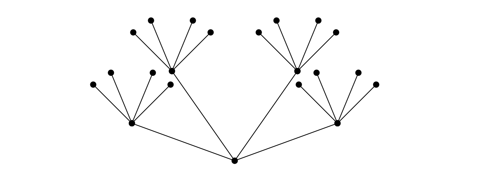
To mathematically express this and connect this with our objective of understanding \(\epsilon_c^{T-n}\), define a path of length \(\ell\) in our computation graph to be a sequence of connected (end-to-end) edges \((p_1, \dots, p_\ell)\) in the computation graph. If \(P_{\ell}\) denotes the set of all such paths of length \(\ell\), then we see that

\[ \epsilon_c^{T-n} = \sum_{\ell=0}^{n}\sum_{(p_1, \dots, p_{\ell}) \in P_{\ell}} G(p_1, \dots, p_{\ell}) \]

where \(G\) is a function that collects gradients from traversing a path \((p_1, \dots, p_{\ell})\).

For example, let \((p_1, p_2, p_3)\) be a path in the LSTM computation graph that starts from the input gate at timestep \(T-1\), goes to the next input gate at timestep \(T\), and then goes to the output of the computation graph at timestep \(T\). Then

\[ G(p_1, p_2, p_3) = \overbrace{ \sum_{\iota=1}^{H} w_{ch}\theta'(a_{\iota}^{T-1}) \sum_{c' = 1}^{C}g(a_{c'}^{T-1})b_{\omega}^{T-1}h'(s_{c'}^{T-1}) }^{\text{input gate}} \overbrace{ \sum_{\iota=1}^{H} w_{c'h}\theta'(a_{\iota}^{T}) \sum_{c'' = 1}^{C}g(a_{c''}^{T})b_{\omega}^{T}h'(s_{c''}^{T}) }^{\text{input gate}} \overbrace{ \sum_{k = 1}^{K}w_{c''k}\delta_{k}^{T} }^{\text{output gate}} \]