Recurrent Neural Networks and the Reber Grammar in PyTorch
Recurrent neural networks are a special type neural network that have been heavily studied for decades towards problems involving sequence prediction, which standard feed-forward neural networks tend not to be that great at. What makes RNNs different is that it processes input sequentially and generates hidden states which are then used in future computations.
Here, we'll offer an overview of RNNs, present an explicit RNN, and then implement an RNN in Pytorch to learn an artificial grammar known as the Reber Grammar. You can find the complete PyTorch code, which we'll also introduce here, in this Github gist.
Recurrent Neural Networks
The aim of recurrent neural networks is to be able to predict unseen sequences of inputs given training from a set of similar sequences of inputs. By a sequence of inputs, we mean a sequence \((x_1, x_2, \dots, x_T)\) of elements, where \(x_i \in \mathbb{R}^n\) for some dimension \(n\). In the typical application of using an RNN for a language model, the \(x_i \in \mathbb{R}^n\) can represent words, which are one-hot encoded. However, we will keep the discussion regarding the sequence elements general, only enforcing that each element in the sequence have the same dimension.
From a very high level, the typical visualization of computing a forward pass through the neural network using such a sequence is via the diagram below.

While this diagram is very simple and somewhat useful for visualization, it doesn't mean much mathematically. Let us go beyond simply showing a colorful diagram and mathematically explain how RNNs work.
For a sequence
the recurrent neural network will compute a sequence of hidden states
and will output a sequence of output values
In many applications, \(m = n\), and we will assume that here for simplicity in our discussion. Depending on the type of recurrent neural network one is employing, there are various ways to compute \(h_t\) and \(y_t\). Typically, the equations are given as
where \(f\), and \(g\) are some functions. Usually in an implementation \(h_0\) is initialized to the zero vector.
Now that we have the general mathematical structure of an RNN settled, we can make things concrete and introduce the most basic kind of RNN. In a vanilla RNN, \(f\) and \(g\) are just feed-forward neural networks. In that case, the computations are given by the equations below.
where
-
\(W \in \mathbb{R}^{d \times n}\) is a trainable weight matrix that acts on the input \(x_{t}\)
-
\(U \in \mathbb{R}^{d \times d}\) is a trainable weight matrix that acts on the hidden states \(h_{t - 1}\)
-
\(V \in \mathbb{R}^{d \times n}\) is a trainable weight matrix that acts on the computed hidden state \(h_t\)
-
\(b_h\), \(b_o\) are trainable biases
-
\(\sigma_o\), \(\sigma_i\) are activation functions (e.g., sigmoid, tanh, etc.).
In addition, \(d\), the dimension of the vector space that the hidden states \(h_t\) live in, is a hyperparameter. One can set it to 5, 10, 1000, etc, but it ultimately depends on what kind of data the RNN is being trained to predict.
An RNN, explicitly
Let us offer an explicit RNN with a simple architecture, and demonstrate how input is computed. Once we go over this simple RNN we will train it to learn the reber grammar, an artificial (fake) grammar invented as a toy sequence prediction problem. Let us design it is as follows.
-
Set \(d = 4\). That is, our hidden states \(h_t\) live in \(\mathbb{R}^4\).
-
Set \(n = 7\). Then we expect our sequence elements \(x_t\) to live in \(\mathbb{R}^7\).
-
Set \(m = n\).
With these hyperparameter and model parameter choices, what does this RNN look like? We can visualize the network computation of one sequence element \(x_t\) in a sequence \((x_1, \dots, x_T)\). Since \(x_t \in \mathbb{R}^7\), let \(x_t = (x^t_1, x^t_2, x^t_3, x^t_4, ,x^t_5 , x^t_6, x^t_7)\). Then this is what the forward pass on \(x_t\) in the RNN would look like:

For simplicity, we omit the biases in the above image. But from this picture, it is easy to see that a vanilla RNN is simply a feed-forward that feeds itself extra values on each forward pass in computing \(x_t\). Namely, when processing the \(t\)-th element in the sequence of data, it feeds itself the current input \(x_t\) and the hidden layer calculations \(h_{t-1}\) from the last time step.
In fact, something else that is evident from the above picture is that you could actually combine \(W\) and \(U\) into one single weight matrix \(W'\) and perform forward pass by concatenating \(x_t\) and \(h_{t-1}\). Later we'll see that this is what we'll do in the code implementation of this network, as is often done in most implementation.
As we will use this network to learn the Reber grammar, we introduce the grammar.
Reber Grammar
The Reber gramma is an artifical grammar introduced by Arthur Reber, a cognitive psychologist, in the 1960s as an example of a experimental learning problem. (According to Reber, the grammar first appeared in his unpublished masters thesis in 1965.) The grammar's rules, which generate legal strings, can be pictured with the following graph.

How do we generate strings from this grammar? We iteratively build a string by traversing the graph. More specifically,
-
For each edge we traverse, we iteratively append the letter corresponding to that edge to our current string in progress.
-
The first letter will always be "B", because there is only one edge to traverse at the beginning.
-
When we are presented with multiple possible edges to travese, we choose the next edge randomly and uniformly.
-
We eventually traverse the last edge "E" at the end, so the last letter is always "E".
An example of a string generated by the above example is BTSSSXSE or BTSXXTVVE, but not BPVPS. BPVPS is not legal because it doesn't finish traversing the graph.
As we said before, the Reber grammar was invented as a learning problem. The problem, which we will also use the RNN to try to solve, can be stated as follows: Suppose we are given many strings which are generated by the Reber grammar. Suppose we do not know how these samples are generated. Can we correctly determine whether or not a new, unseen string is a legal string generated by the grammar?
Interestingly, while the Reber grammar became widely discussed in the early literature on neural networks, Reber actually created this grammar to test on humans. Reber was interested in something called implicit learning; the idea is that there are certain things we, as humans, learn, but cannot exactly explain how we learned it (e.g. riding a bicycle) or sometimes we learn unintentionally or unconsciously (hence "implicitly"). To test this, Reber invented this grammar and gave participants different instructions on how to predict if a new, unseen sequence was valid or not; some were given instructions, some were to learn implicitly. He demonstrated that participants who were given instructions were worse at predicting valid examples than the ones that learned implicitly, giving evidence to the idea that humans can learn implicitly.
While Reber tested humans on this learning problem, we will be doing the same thing but to an RNN.
In order to do this, we will first implement the graph in code. It is not that hard.
graph = {
    0: [(1, "b")],
    1: [(2, "t"), (3, "p")],
    2: [(2, "s"), (4, "x")],
    3: [(3, "t"), (5, "v")],
    4: [(3, "x"), (6, "s")],
    5: [(4, "p"), (6, "v")],
    6: [(-1, "e")],
}
Here, 0 denotes the initial state and -1 denotes the terminal state. Next, we'll need to be able to generate strings from this graph. Hence we implement a random traversal of this graph (uniform probability when presented with multiple edge options)
import random

def randomly_traverse_graph(graph):
    curr_node = 0
    sentence = ""
    while True:
        next_states = graph[curr_node]
        if len(next_states) > 1:
            next_state = random.choice(next_states)
        else:
            next_state = next_states[0]
        next_node = next_state[0]
        next_letter = next_state[1]

        sentence += next_letter
        curr_node = next_node
        if curr_node == -1:
            break

    return sentence
That is basically it in terms of implementing the Reber grammar and generating examples from the grammar.
Reber Grammar Problem Statement and Data Representation
Now that we have introduced the Reber grammar, we will introduce the problem statement that we will have the RNN attempt to solve:
Suppose we are given many examples generated by the Reber grammar and we are unaware of the rules in which these strings are generated. Given a new, unseen string, can we determine if it was generated by the Reber grammar?
Our training and evaluation plan for the RNN will be as follows.
-
Generate many examples to obtain a training and test set. Additionally, append invalid, non-Reber strings to the test set for later evaluation.
-
Train the RNN.
-
The RNN will operate in the following way: It will process a string sequentially by traversing each letter. On traversing a single letter, it will output a vector of probabilities. This vector will tell us how likely any of the letters in our alphabet ("BTSXPVE") is most likely to appear next.
-
Given the trained RNN, present it with a valid Reber string from the test set. Traverse each letter and present it to the model sequentially. If either of the model's two highest next letter predictions match the actual next letter, then the model is said to be correct. Otherwise, it is incorrect. If it processes the whole test string correctly, then the model passes on the valid test example.
-
Given the train RNN, also present it with an invalid Reber string from the test set. Traverse each letter and present it to the model sequentially. If either of the model's two highest next letter predictions do not match the actual next letter, then the model is said to be correct. Otherwise, it is incorrect. If it processes the whole test string correctly, then the model passes on the invalid test example.
At this point, we have one question: How will we design this RNN? Answer: We already did. The RNN introduced in the previous section will be the exact same architecture that we will use for this problem.
The next question we'd have that this point, which we now turn to: How do we want to represent our input data (Reber strings) for our model? We'll represent a string as a sequence of one-hot encoded vectors, where each one-hot encoded vector specifies which letter in our alphabet ("BTSXPVE") it represents. Because our alphabet contains 7 characters, these one-hot encoded vectors will live in \(\mathbb{R}^7\).
Let us give an example. For the input string "BPVPSE", we'd represent it as the sequence of vectors in \(\mathbb{R}^7\)
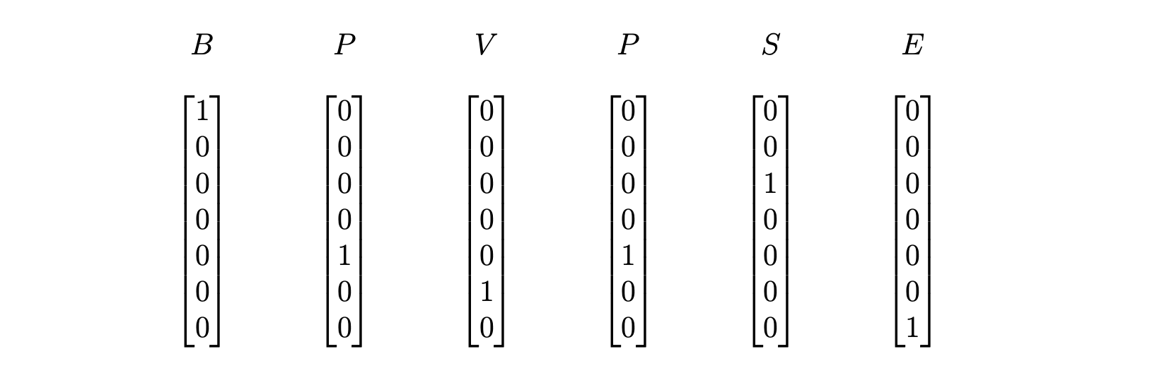
We can implement the logic of converting a Reber string to a one_hot encoded vector as below
def convert_string_to_one_hot_sequence(reber_string):
    sequence = []
    alphabet = "btsxpve"
    for letter in reber_string:
        vector = [0 for _ in range(len(alphabet))]
        for ind, elem in enumerate(alphabet):
            if elem == letter:
                vector[ind] = 1
                break
        sequence.append(vector)
    return sequence
Defining the RNN in Pytorch
We now implement the RNN we proposed earlier from scratch in Pytorch. Pytorch has an RNN class but we'll just implement the RNN ourselves.
The architecture in Pytorch is rather straightforward. Also, in our implementation, when we are computing a forward pass we will simply concatenate the input with the previous hidden state, so that we only have to worry about one weight matrix instead of two weight matrices \(W\) and \(U\).
import torch
import torch.nn as nn


class RNN(nn.Module):
    def __init__(self, input_size, hidden_size, output_size):
        super(RNN, self).__init__()
        self.hidden_size = hidden_size
        self.hidden_transform = nn.Linear(input_size + hidden_size, hidden_size)
        self.output_transform = nn.Linear(hidden_size, output_size)
        self.tanh = torch.tanh
        self.sigmoid = torch.sigmoid

    def forward(self, input, hidden):
        combined = torch.cat((input, hidden), 1)
        hidden = self.hidden_transform(combined)
        hidden = self.tanh(hidden)
        output = self.output_transform(hidden)
        output = self.sigmoid(output)
        return output, hidden

    def initHidden(self):
        return torch.zeros(1, self.hidden_size)
This allows us to implement our model and compute a forward pass as below.
rnn = RNN(7, 4, 7)

sequence = [torch.randn(1, 7) for _ in range(10)]
hidden = rnn.initHidden()
outputs = []

# Perform a forward pass and collect each prediction
for elem in sequence:
    output, hidden = rnn(elem, hidden)
    outputs.append(output)
Preparing Training Data
In order to use our model, we need to prepare some training data \(\{\dots, (x_t, y_t), \dots\}\). As we explained earlier, we know that the input to our model \(x_t\) will be a sequence \((x_1^t, \dots, x_n^t)\), where \(x_i^t \in \mathbb{R}^7\) is a one-hot encoded vector. Additionally, the output of our model will be a vector in \(\mathbb{R}^7\) representing probabilities. Thus, how exactly should we prepare training data?
Let us give an example. For the legal Reber string "BPVPSE", we'd want the model to output the following vectors.
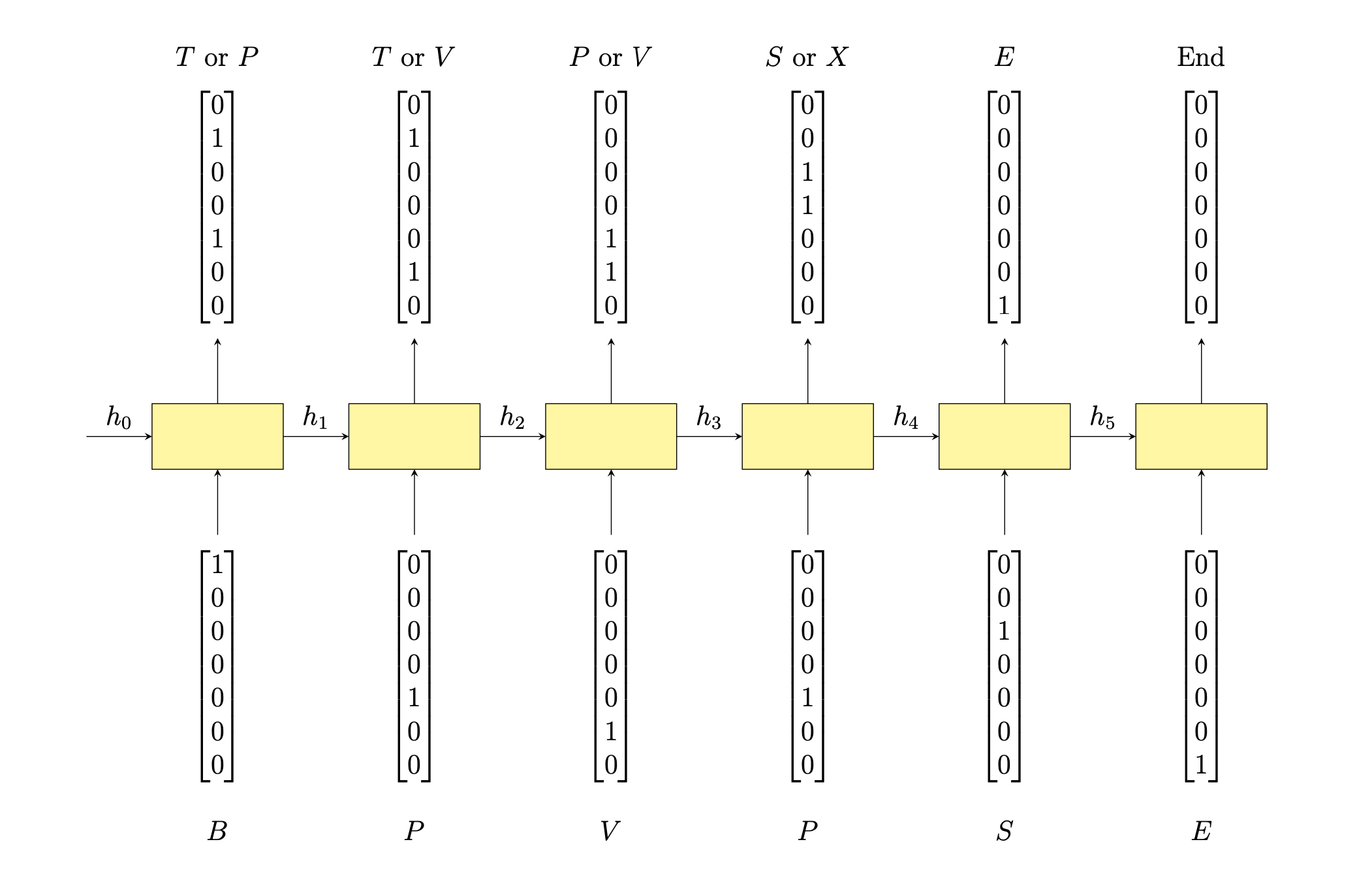
Hence, for the input string \(BPVPSE\), the target value in our test set would be the sequence of boolean vectors as above. That way, the model would correctly indicate, via 1s and 0s, what letters could possibly appear at each stage in a Reber string, and therefore it could learn the grammar.
Here, we write a Python function that maps a Reber string to its target input.
def generate_training_target(sequence):
    alphabet = "btsxpve"
    curr_node = 0
    targets = []
    for letter in sequence:
        # Go to the next node in the graph
        next_state = None
        for option in graph[curr_node]:
            if letter == option[1]:
                next_state = option
                break
        if next_state is None:
            print(f"Error, this sequence is invalid at this {letter=}: {sequence=}")
            break
        # Look at the next node options
        next_node = next_state[0]
        target = [0 for _ in range(len(alphabet))]
        if next_node == -1:
            targets.append(target)
            break
        # One hot encode the next possible
        for option in graph[next_node]:
            for ind, letter in enumerate(alphabet):
                if letter == option[1]:
                    target[ind] = 1
                    break
        curr_node = next_node
        targets.append(target)
    return targets
Calling this function on the Reber string we used above returns the expected vectors.
[ins] In [107]: generate_training_target("bpvpse")
Out[107]:
[[0, 1, 0, 0, 1, 0, 0],
 [0, 1, 0, 0, 0, 1, 0],
 [0, 0, 0, 0, 1, 1, 0],
 [0, 0, 1, 1, 0, 0, 0],
 [0, 0, 0, 0, 0, 0, 1],
 [0, 0, 0, 0, 0, 0, 0]]
Next, another function we'll need in order to generate training data is this simple function below.
This functions allows us to create a dataset of Reber strings, controlling the minimum and maximum string lengths.
Note that we are using the function randomly_traverse_graph that we defined earlier.
def generate_n_samples(graph, num_samples, min_length, max_length):
    samples = set()
    while len(samples) < num_samples:
        sample = randomly_traverse_graph(graph)
        if len(sample) < min_length or len(sample) > max_length:
            continue
        samples.add(sample)
    samples = list(samples)
    return samples
Training in Pytorch
Now that we have a training plan and way to generate our training data, we move onto training the RNN in Pytorch.
Training RNNs has historically been very difficult for researchers. The most obvious way to train RNNs is through applying a strategy similar to the backpropagation algorithm used for feed forward neural networks. This works in theory, e.g., (Werbos, 1990), and is known as the Back Propagation Through Time method. But while this works in theory, and explicit update formulas can be written, the recursive nature of RNNs cause the resulting formulas to have many products, which grows with the number of time steps used in training data. As a result, gradients computed through BPTT tend to either vanish or explode (Bengio et. al.).
There are various techniques one can employ to avoid the vanishing gradient problem in RNNs, such as only training on the last \(k\) time steps, etc. The most promising work towards addressing this problem was through the invention of the LSTM model (Hochreiter et. al., 1997).
Here, we will employ the equivalent of the naive backpropagation through time method, since it doesn't cause any issues for our data. Our training function is given as below.
import torch.nn as nn

def train_one_example(
    rnn: nn.Module,
    target: list[torch.tensor],
    input_sequence: list[torch.tensor],
    learning_rate: float,
    criterion,
):
    rnn.zero_grad()
    hidden = rnn.initHidden()
    loss = 0
    for i in range(len(input_sequence)):
        output, hidden = rnn(input_sequence[i], hidden)
        loss += (1 / len(input_sequence)) * criterion(output, target[i].float())

    loss.backward()

    # Add parameters' gradients to their values, multiplied by learning rate
    for p in rnn.parameters():
        p.data.add_(p.grad.data, alpha=-learning_rate)

    return output, loss.item()
We can then use this function to write a function that trains the model on an entire training dataset for a certain number of epochs.
import torch.nn as nn

def train(
    rnn: nn.Module,
    epochs: int,
    training_data: list[tuple[torch.tensor]],
    learning_rate: float,
    criterion,
):
    for _ in range(epochs):
        epoch_loss = 0
        for ind in range(len(training_data)):
            sequence, target = training_data[ind]
            output, loss = train_one_example(rnn, target, sequence, learning_rate, criterion)
            epoch_loss += loss
        print(epoch_loss)
We now have everything we need to train our model on the Reber grammar data. The following code does exactly that. In our code, we're using
- A learning rate of 0.4
- 400 samples for training and testing, using strings ranging from length 30 to 52
- 10 epochs
- BCE (Binary cross entropy)loss function
import torch.nn as nn

# Specify model settings
n_hidden = 4
input_size = 7
output_size = 7
rnn = RNN(input_size, n_hidden, output_size)

# Specify dataset settings
num_samples = 400
data = generate_training_data(graph, num_samples, 30, 52)
training_data = data[: int(0.8 * num_samples)]
test_data = data[int(0.8 * num_samples) :]

# Specify training settings
learning_rate = 0.4
epochs = 10
criterion = nn.BCELoss()
train(rnn, epochs, training_data, learning_rate, criterion)
Running this code, you should see something like
97.66354854404926
45.04029807448387
28.23289054632187
18.152766678482294
13.75518929772079
11.260628033429384
9.576107319444418
8.345648445189
7.399222897365689
Evaluation
Now that we can train the model, how do we evaluate its performance? As we said before, the goal is for the model to always correctly predict legal next-letter options when traversing a Reber string. In this way, the model can learn to validate legal reber strings and reject invalid strings.
To do this, we can write a function that evaluates the model given on test example from the testing set. As the model is iteratively fed each one-hot encoded letter, it announces what it thinks to be the next two possible letters. If these two predictions match what true next letter, then the model has passed the test. Otherwise, it fails.
def eval_one_input(rnn: nn.Module, input: list[torch.tensor]) -> bool:
    hidden = rnn.initHidden()
    for ind, letter in enumerate(input):
        if ind == len(input) - 1:  # the model succeeded
            continue
        prediction, hidden = rnn(letter, hidden)
        _, indices = prediction.sort()
        next_letter = input[ind + 1][0]
        if int(next_letter.nonzero()) not in indices[0][-2:]:
            print(
                f"Network incorrectly predicted {prediction=} at {ind=}, next letter was {next_letter=}"
            )
            return False
    return True
We can then use this function to build our main evaluation function, which tests the model across the entire test dataset and summarizes the pass rate of the model.
def eval_model(rnn: nn.Module, test_data: list[tuple[torch.tensor]]) -> None:
    rnn.eval()
    num_passed = 0
    for sequence, _ in test_data:
        reber_string = convert_one_hot_sequence_to_string(sequence)
        passed: bool = eval_one_input(rnn, sequence)
        if passed:
            print(f"Network passed on {reber_string=}")
            num_passed += 1
        else:
            print(f"Network failed on {reber_string=}")

    pass_rate = num_passed / len(test_data)
    print(f"Overal pass rate: {pass_rate=}")
We can then call the above function eval_model on our trained RNN. Doing so yields output to
stdout as below.
...
Network passed on reber_string='btsxxtttvpxtvve'
Network incorrectly predicted prediction=tensor([[1.1079e-03, 6.1265e-02, 1.6927e-01, 1.5435e-01, 9.5694e-05, 7.1114e-01,
         1.0911e-02]], grad_fn=<SigmoidBackward0>) at ind=1, next letter was next_letter=tensor([0, 1, 0, 0, 0, 0, 0])
Network failed on reber_string='bpttvpxttvpxtvve'
Network passed on reber_string='btxxvpxtttvve'
...
Overal pass rate: pass_rate=0.7607142857142857
You can play with the model parameters and training examples to obtain a pass rate of 1.0. For me, I used the following parameters to achieve a perfect pass rate on a small dataset.