Phrased-Based Translation Model and Decoder
While IBM models were effective at word alignment, they don't produce the best translation models, since in order to use it for translation one must perform a word-by-word approach. However, when it comes to translation, this isn't the best approach.
For starters, a word-by-word approach does not take into the context that each word appears in. For example, suppose we are machine that has seen a translation of "Tienes hambre?" and we are now given "Tienes tarea?" Following a naive maximum-likelihood, word-by-word approach, since we know that "Tienes hambre?" -> "Are you hungry?", we might end up with a translation "Tienes tarea?" -> "Are you homework?" when it should be "Do you have homework?". Conversely, if we flipped our examples we might end up translating "Tienes hambre?" -> "Do you have hungry?"
It turns out that it is actually easier to translate from a source language to a target language if we perform translation by examining local groups of words--which we call phrases--based on how often we see them together and on what group of words in the target language they tend to be aligned to.
In order to formulate this, consider more generally the fact that what we seek in terms of a translation model is a conditional probabilistic model \(p(\mathbf{e} | \mathbf{f})\) where \(\mathbf{e}\) represents a target language sentence and \(\mathbf{f}\) represents our source language sentence. This is because if we can obtain such a model, we can compute
in order to find an optimal translation of a given source language sentence \(\mathbf{f}\). Note that by a simple application of Bayes theorem, we can write
The last expression offers a nice interpretation to our task at hand. It means we must develop a translation model going into the reverse direction (target language to source) and a language model \(p(\mathbf{e})\), which from hereon we denote as \(p_{LM}\). As a side note, this formulation of \(p(\mathbf{e}| \mathbf{f})\) is known as the Noisy Channel model, as it can be thought of more generally as attempting to decode a given message over a noisy channel.
Phrase-Based Model
At this point, we now introduce the phrased-based translation model \(p(\mathbf{f}| \mathbf{e})\). Whereas before with IBM models we were partitioning our sentences word-by-word \(\mathbf{e} = (e_1, \dots, e_n)\), with the phrase-based approach we partition the sentence by groups of words, known as phrases:
where in the above expression \(I\) is the number of phrases we divide our sentence into. Note that phrases are denoted with an overline bar, and that we will write \(\mathbf{e}^I\) to emphasize via \(I\) that \(\mathbf{e}\) is a sentence that has some partition \((\overline{e}_1, \dots, \overline{e}_I)\) relevant to the given context.
With that said, the phrase-based translation model is given by the expression below.
where
- \(\phi(\overline{e} | \overline{f})\) is a phrase translation model that models the probability a French phrase is translated by an English phrase (Note that the phi symbol is used for "phrase")
- \(\text{start}_i\) denotes the index in the string \(\mathbf{f}\) that phrase \(\overline{f}_i\) starts at
- \(\text{end}_i\) denotes the index in the string \(\mathbf{f}\) that phrase \(\overline{f}_i\) ends at
- \(d(\text{start}_i - \text{end}_{i-1} - 1)\) is a distortion model that takes into account reordering that can occur when performing translation at the phrase level.
For an initial approach, we can use a simple exponential model \(d(x) = \alpha^{|x|}\) to model distortion.
The above model then leads to our calculation that
The above model is how the first successful phrased-based translation model was proposed by Koehn, Och, and Marcu in their 2003 paper Statistical Phrase-Based Translation. In the paper, they also introduce the idea of weighting the language model, and setting this weight parameter close to 0.25, to achieve their desired performance. It turned out later that the model could be even further customized by weighting different parts of the function as well.
To do this, one can specify parameters \(\lambda_{\phi}\), \(\lambda_{d}\), and \(\lambda_{LM}\) to control how the phase translation model, distrotion model, and language model contribute to the overall translation model, as follows.
This formulation of the translation model becomes useful once we additionally notice that \(\mathrm{argmax}_{\mathbf{e}} p(\mathbf{e}, \mathbf{f}) = \mathrm{argmax}_{\mathbf{e}} \log(p(\mathbf{e}, \mathbf{f}))\). Doing so, we can then see that we actually just need to maximize the expression below.
which is actually really nice. The model is now a linear combination of several different features (phrase translation probability, distortion probability, language model). Further, in an implementation context, we can avoid numerical underflow by working in the logarithmic space, which is likely to occur because probability can often be very small numbers. And from this perspective, we can additionally tack on other statistical features and weight them with different parameters to customize the model even further.
In order to use this model in an implementation context, one has to actually create the phrase translation table \(\phi(\overline{e},\overline{f})\). What is nice about this is that this table can be constructed given a parallel corpus dataset, which is usually performed by using a word alignment model. Once this phrase translation table is constructed, we can use the model to actually perform decoding.
Phase Based Decoding: Hypothesis
Using the translation model introduced, we can design a decoding algorithm which employs a beam search that finds the best possible translation of a sentence, so long as we have access to
- a phrase translation table \(\phi(\overline{e} | \overline{f})\)
- a language model \(p_{LM}(\mathbf{e})\)
The main idea of the beam search will be to (1) construct a set of translation options of \(\mathbf{f}\) into English by partitioning \(\mathbf{f}\) into phrases and then (2) declare the most optimal translation to be whichever partition optimizes our phrase-based probability model. This most optimal translation will then be our sentence \(\mathbf{e}\).
In order to easily construct a set of translation options of \(\mathbf{f}\), we'll need to use a data structure known as a hypothesis. A hypothesis of \(\mathbf{f}\) is a node in a linked list that translates one phrase \((f_{i}, f_{i+1}, \dots, f_{i + n})\) in \(\mathbf{f}\) into an English phrase. Forming a linked list of a set of hypotheses then allows us to propose one sentence translation option of \(\mathbf{f}\) into English.
To motivate the hypothesis data structure, let us given an example of such a linked list.
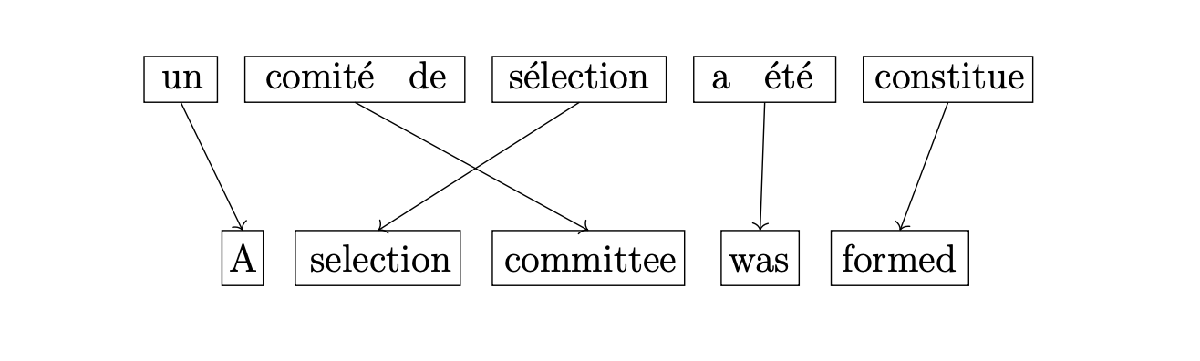
Consider the French sentence un comite de selection a ete constitue,
and suppose we are an all-knowing French-English translator attempting to translate this into English.
We could translate the sentence into English and map the phrases between the sentences like so.
Since we are an all-knowing French-English translator, we know the first thing to translate
is un which translates to the English word a. We'd write this down as a hypothesis like so.
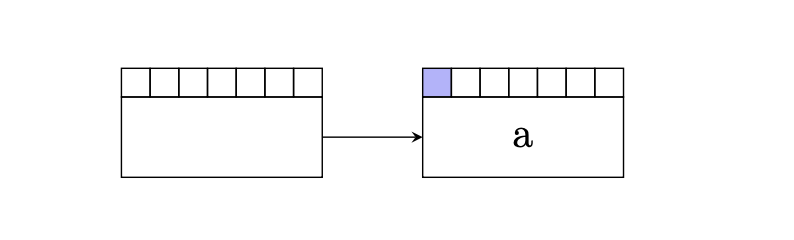
Here we'll note a couple of things about the above diagram.
- We initialize this linked list data structure with an empty hypothesis. This is emphasized in the above diagram with the empty hypothesis on the left.
- We color in the first square to indicate the first word in our foreign sentence has been translated. Later, we'll use a different color to differentiate between the most recently translated words by a hypothesis.
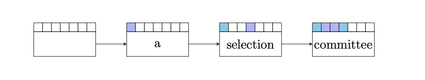
Next, we see comite de selection, which roughly translates to committee of selection. Because we're all-knowing, we know
that a better translation is actually selection committee. Thus, we'd know that it is better to first
translate the French phrase selection to the English phrase selection

and then we translate the phrase comite de to the English word committee.
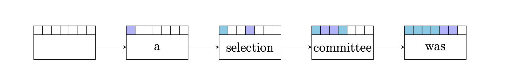
At this point, we have 3 words left in the foreign sentence to translate, and we can see that the next best thing to translate would be a ete, because this phrase roughly translates to the English word was. We write this down as a hypothesis.
Finally, we have one word left to translate; we see constitute, which from the context of the sentence we could translate to formed. This is our last hypothesis.
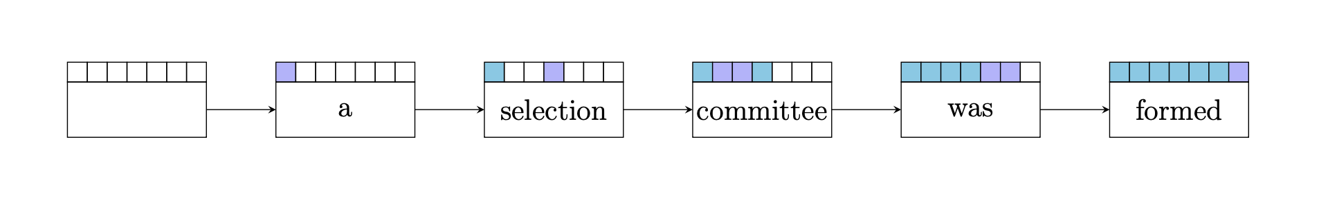
Traversing the linked list left from right gives us our English translation.
From this example, we can see that the point of the hypothesis data structure is to enable us to create a linked list data structure that iteratively translates \(\mathbf{f}\), one phrase at a time, into English. To summarize, this linked list data structure is constructed as follows.
-
Each new hypothesis we append to the linked list will attempt to translate one phrase of \(\mathbf{f}\) only using words in \(\mathbf{f}\) that haven't already been translated by any of the previous hypotheses.
-
Each time we add a node to the list we have less words to translate. Hence building such a linked list will always terminate.
In our example, we knew what the final translation was going to be. In general, what we will have to do is construct all possible translation options, by building many, many hypotheses and linked lists, and then selecting whichever linked list translation maximizes our probability model.
Constructing translation options: Computational intractability
Thus at this point, all we need to do is construct our set of possible phrase translations of the sentence \(\mathbf{f}\). It turns out that this is not realistic.
Doing this requires running a horribly expensive recursive algorithm, with beyond worse than exponential runtime with respect to sentence length. To demonstrate this, let us count the number of translation options we would in theory need to construct. To do this, we will need to leverage the following Python function.
def all_remaining_subphrase(words_translated, sentence):
    subphrases = []
    for window_size in range(1, len(sentence) + 1):
        i = 0
        while i + window_size <= len(sentence):
            subphrase = list(range(i, i + window_size))
            add = True
            # check if subphrase contains words we already translated.
            for word in words_translated:
                if word in subphrase:
                    add = False
                    break
            if add:
                subphrases.append(subphrase)
            i += 1
    return subphrases
For simplicity, this function simply works on integers, versus actual words and sentences, but the point of this function is so that we can call it and obtain functionality as below.
[ins] In [45]: all_remaining_subphrase([], [1, 2, 3, 4])
Out[45]:
[[0],
 [1],
 [2],
 [3],
 [0, 1],
 [1, 2],
 [2, 3],
 [0, 1, 2],
 [1, 2, 3],
 [0, 1, 2, 3]]
def count_hypothesis_options(words_translated, sentence):
    count = 0

    if len(words_translated) == len(sentence):
        return 1

    for subphrase_inds in all_remaining_subphrase(words_translated, sentence):
        count += count_hypothesis_options(words_translated + subphrase_inds, sentence)

    return count
[ins] In [40]: for i in range(1, 12):
          ...:     print(count_hypothesis_options([], list(range(i))))
          ...:
1
3
11
49
261
1631
11743
95901
876809
8877691
Since the binomial coefficient itself involves factorials, we see that this algorithm would be at least \(O(n!)\) with respect to sentence length. One can see how fast this sequence grows by viewing this precomputed table of the first 200 values of this sequence.
Fortunately, a lot of the translation options we'd construct in this fashion turn out to be unnecessary and redundant, and there are a few strategies we can employ to throw away translation options that are weak or redundant. Doing this reduces the number of translation options we have to sift through.
Recombination
There are two basic strategies we can implement to reduce our search space.
- Recombination
- Pruning
Recombination involves throwing away duplicate translation options whenever possible. When we find that we are working on two duplicate translation options, we simply throw away the weaker option using the phrase-based model for scoring.
When are two translation options rendundant? We'll answer this with a few examples.
Suppose we are translating the Spanish sentence Este es la verdad. Then an example of two
redundant translation options would be as below.
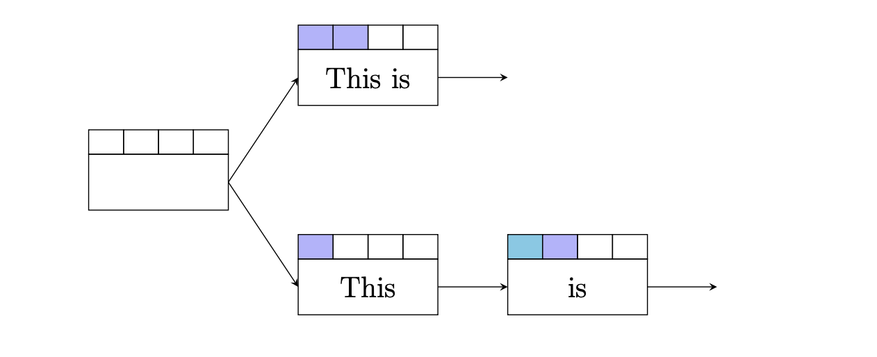
In this case, each translation option has so far translated the same exact foreign words, and their English translations are identical. Thus we can safely drop whichever translation option has the worst score.
However, recombination can be applied even when the English translations aren't exactly the same. In this example, the two translation options translated the first word differently, but the last two words translated are the same.

Assuming a trigram language model (thus the language model cares about the last two words when performing scoring), which we do in this case, the rule for recombination is as follows.
- Both translation options must have the so far translated the same foreign words.
- The last two English translations in both translation options must match.
- The same last foreign word translated must be the same.
Pruning
Performing recombination reduces duplicates, but it turns out that there will still be too many translation options. One way to address this issue is to assemble our translation options in a specific way, which involves placing our hypotheses during decoding into stacks.
During decoding, we will create a number of stacks in the following way.
- For decoding a sentence \(\mathbf{f}\) with \(n\)-many words, we will create \((n + 1)\)-many stacks.
- Stack \(i\) will contain all hypotheses that have translated \(i\)-many words.
Below is an illustration of how we would assemble our translation options into these stacks during decoding.
In this example, we are trying to translate the sentence
ella no quiere comer antes de la fiesta. In the picture we draw 4 stacks, although of course in this case there are actually more stacks.

In the first column, we have translated exactly one word from the foreign sentence into English, in the second we have
translated two foreign words, etc. Note that when
building these stacks during decoding, you don't have to
translate in a monotone order (i.e. starting at the beginning of the foreign sentence). In fact, that is not desirable, as sometimes
translating phrases requires going out of order (e.g. think of our earlier example where we translated
comite de selection -> selection committee).
The purpose of putting our hypotheses into stacks is so that we can perform pruning. Pruning allows us to cap the number of hypotheses allowed in each stack. This number can range from 10, 100, 1000, etc., and is known as the stack size or beam size. This, in essence, is why we call this a beam search, since we are building a large search space but we are limiting the number of search options we will allow ourselves to sift through.
By pruning, we can implement a phrase-based decoder with the following pseudocode.
# initialize stacks
stacks = []
for _ in range(len(foreign_sentence) + 1):
    stacks.append([])
stack[0].append(inital_hypothesis)

for stack in stacks:
    for hypothesis in stack:
        for phrase in all_phrase_options(hypothesis): # expand hypothesis
            if phrase in language_model:
                new_hypothesis = Hypothesis(phrase)
                new_hypothesis.prev = hypothesis
                # try to recombine, otherwise add to stack
                if can_recombine:
                    recombine(hypothesis, new_hypothesis)
                else:
                    # add new hypothesis, possibly prune stack
                    stack[num_words_translated].append(new_hypothesis)
                    if len(stack) > max_stack_size:
                        prune_stack(stack)
What remains to be answered at this point is: how do we cap the stack size? There are many heuristics on how to prune the hypotheses stacks. The method employed in the original Koehn et. al. paper was to cap the stack size by keeping the hypotheses that have the best estimated future score. That is, whenever a stack reaches a limit during decoding, and we want to add a new hypothesis to it, we must either
- replace an existing hypothesis in the stack with the new hypothesis if the existing has a higher future cost than the new hypothesis
- throw away the new hypothesis we're trying to add, and leave the stack alone
The choice we make depends on the estimated future cost of all the hypotheses in the stack and the new hypothesis. We keep whichever future cost is lower.
Estimated Future Cost
To compute the future cost of a hypothesis, we need to look at what foreign words have not yet been translated by a hypothesis. For example, consider this hypothesis.
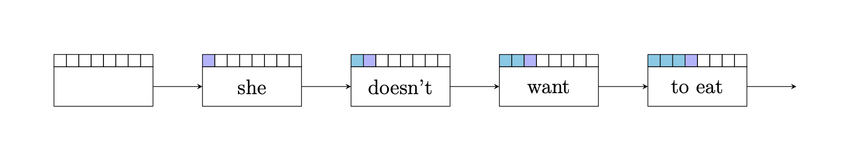
In this example, we see that the foreign words antes de la fiesta have yet to be translated by our hypothesis.
However, we can have slightly more complicated hypotheses that jump around the sentence. For example, consider
this hypothesis.
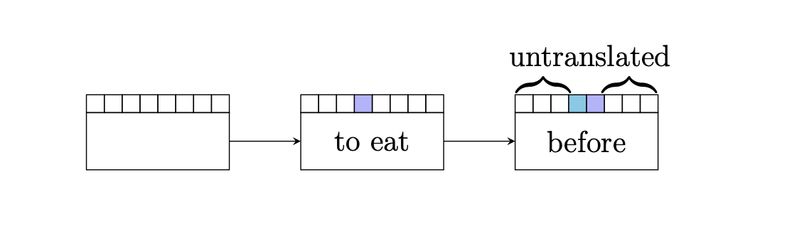
We see that there are actually 2 phrases of foreign words that have yet to be translated.
In any case, what is clear is that for any hypothesis, there exist a certain number of untranslated phrases in the foreign sentence that need to be translated via additional hypotheses. Therefore, the way we compute the future cost is as follows: For each remaining untranslated foreign phrase, we
- Find the cheapest English translation of the phrase (there could be many; choose the one which the phrase translation model scores the best).
- Compute the language model cost of the English translation.
- Multiply these quantities (or add these quantities, if working in log-space). The result is the estimated future translation cost for this foreign phrase.
- If the hypothesis has multiple untranslated foreign phrases, perform this procedure on each foreign phrase and add up the cost.
This estimation of the future cost actually ignores the distortion cost, but experiments show that that's mostly okay to ignore. Additionally, ignoring the contribution of the distortion also allows us to precompute all of these values into a future cost table. Then at decoding time, we can reference this table at any time to estimate the future cost translation for a hypothesis